Sometimes in our data, we want to see the effectiveness of other variables or the impact of multiple data for the sales.
\(\widehat{Y} = 3.337+168.582x_{1}+ 67.151x_{2} \)The given equation use for the multiple linear regression.
Based on our data from the previous lesson in part II, we only have one predictor which is the online advertising cost. Now, as for experimentations, we want to add the variable Free Shipping. With that said, we want to see if adding free shipping will give a big impact on the Monthly E-commerce Sales as well.
| Store | Monthly E-commerce Sales (in $1000) | Online Advertising Cost (in $1000) | Free Shipping |
|---|---|---|---|
| 1 | 370 | 2.3 | No |
| 2 | 311 | 1.7 | No |
| 3 | 620 | 3.0 | Yes |
| 4 | 910 | 5 | Yes |
| 5 | 500 | 2.9 | Yes |
| 6 | 520 | 2.5 | Yes |
| 7 | 600 | 3.4 | Yes |
| 8 | 830 | 4.3 | Yes |
 library("car") #You need to install the package
 Sales<-c(370, 311, 620, 910, 500, 520, 600, 830)
 Advertising.Cost<-c(2.3, 1.7, 3.0, 5, 2.9, 2.5, 3.4, 4.3)
 Free.Shipping<-c(0,0,1,1,1,1,1,1)
 mod<-lm(Sales~Advertising.Cost + as.factor(Free.Shipping))
 summary(mod)
Now let’s see the significance of the free shipping. As you can see, the free shipping seems not to really impact the overall monthly e-commerce sales since its p-value is greater than 0.05. This is because if you see our datasets, the sales really actually affected (driven) by the increases in advertising costs.
Note: In reality, free shipping should attract more customers which means more sales but for the sake of this lesson I showed you the opposite result :-).
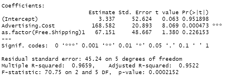
Above is the equation for multiple linear regression
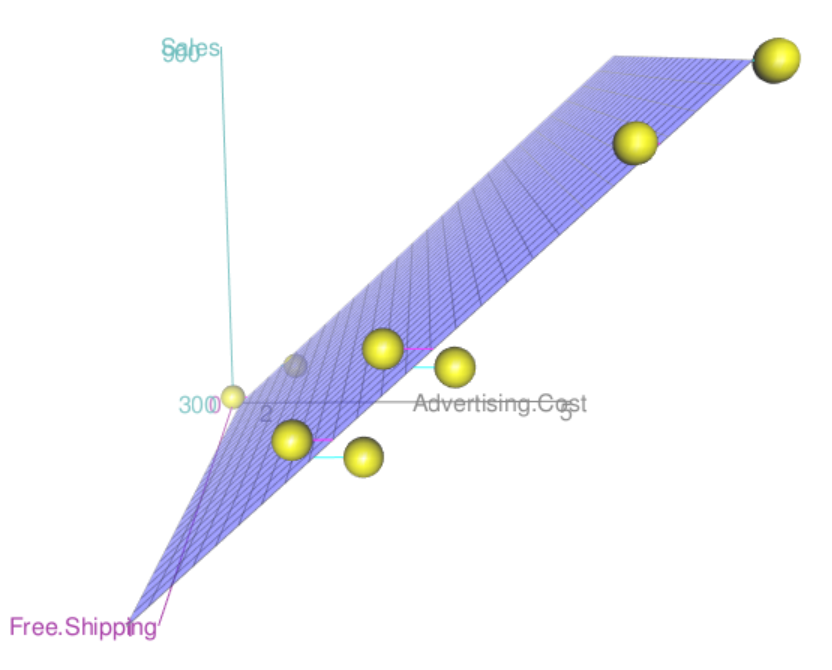
Now, let see the 3d plot using scatter3d() function
scatter3d(x=Free.Shipping, y=Advertising.Cost,z = Sales)